Nowadays, we hear about artificial intelligence (AI) everywhere, it affects all sectors… and cybersecurity is not to be left out! According to a global benchmark published by CapGemini in the summer of 2019, 69% of organizations consider that they will no longer be able to respond to a cyber-attack without AI. Gartner places AI applied to cybersecurity in the top 10 strategic technological trends for 2020.
Throughout two articles, we will explore AI’s capabilities, specifically those pertaining to Machine Learning for cybersecurity. In this first article, we will go through each stage of a Machine Learning project focused on a cybersecurity use scenario: the exfiltration of data from the IS, on a very simplified case. We have chosen a case study, but the concepts of this article are applicable to all Machine Learning projects and can be transposed to any other use case, most notably cyber.
First of all, what are we talking about?
The term Artificial Intelligence (AI) includes all the techniques that allow machines to simulate intelligence. Today, however, when we talk about AI, we very often talk about Machine Learning, one of its sub-domains. These are techniques that enable machines to learn a task, without having been explicitly programmed to do so.
For us cybersecurity professionals, this is a good thing: we often find it difficult to describe explicitly what it is we want to detect! Machine Learning then provides us with new perspectives, that have already many application cases, of which the main ones are illustrated hereunder:
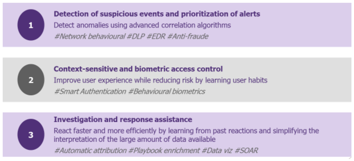
The example of a use case for ML-enhanced cybersecurity: the DLP
To illustrate the contribution of Machine Learning to cybersecurity, we have chosen to focus on the fraudulent extraction of data from a company’s information system. In other words, the case of DLP (Data Leakage Prevention), an issue encountered by many companies. We want to detect suspicious outbound communications in order to prevent them from happening.

«Very well but… how do we identify a suspicious communication? »
By large traded volumes? By a strange destination? By an unusual connection time?
In reality, our problem is complex to explain and what we need to assess is likely to change over time. Therefore, by using only static detection rules, our security teams find it difficult to be exhaustive. They can play on the thresholds of these rules to refine the detected elements, but unfortunately still find themselves with a large number of false positives to deal with.
We understand that the Machine Learning as we defined it previously can be useful here. What if we try it?
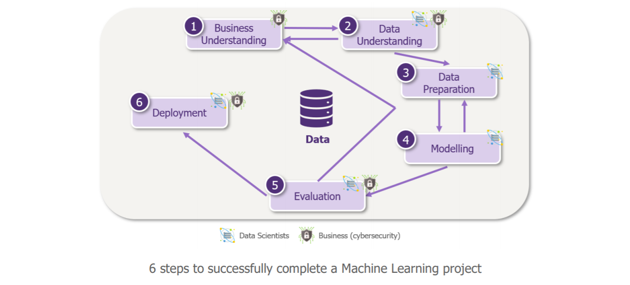
Step 1: Clarify the need
That is what we just did!
Step 2: Choose the data
When we hear the words Machine Learning, we usually must understand “data” to feed the algorithms. Lots of data, and of good quality!
When asking where to get useful data for our data exfiltration case to our requesting business (which for once is cybersecurity!), the web proxy stands out as the big winner: it sees almost all the traffic that comes out through the IS. So, we recovered its logs and they look like this:

« This all seems quite complicated…»
Data scientists have indeed enough reasons to get lost: on the one hand, the whole thing is not easily understandable, and on the other hand, after consultation with the cybersecurity business, not all fields are really useful for our use case. We therefore selected some of them with the cybersecurity business before continuing.

The result is easier for data scientists to use!
Step 3: prepare the data
Data scientists can now “explore the data” in order to ensure optimal learning of the algorithm. Here, they give us a surprising element in the distribution of our requests according to their upload volume. Since we want to detect data exfiltration, this variable is of particular interest to us.
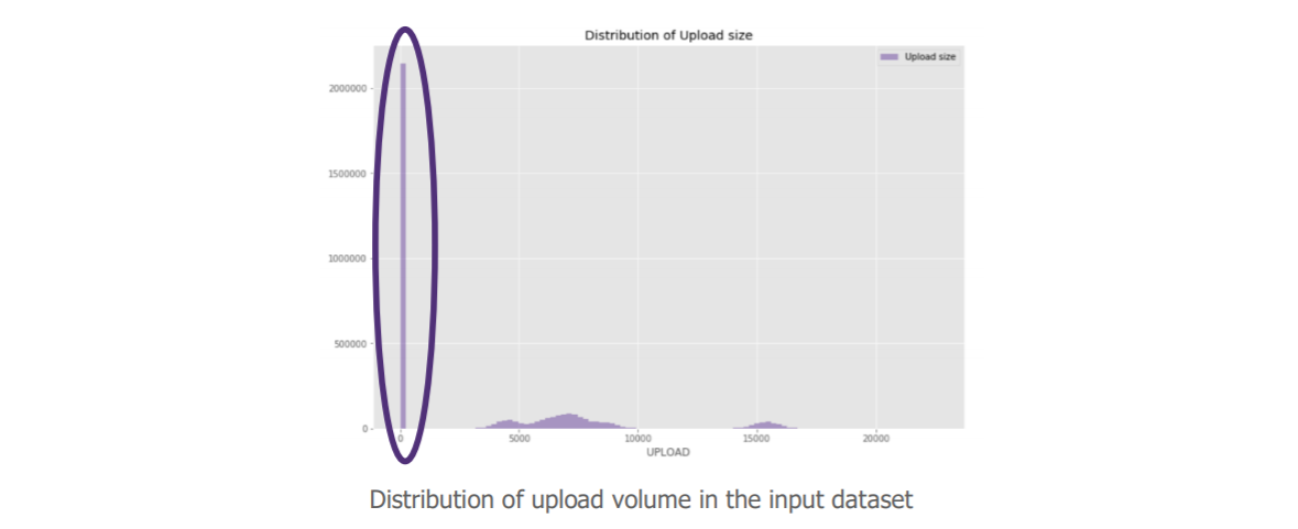
The value of our variable is not distributed, we even have a very high volume at 0.
“But still, there are a lot of these requests with a null upload volume; is it really relevant to keep them in our case? “.
Indeed, after discussion with the cybersecurity business, it appears that these data do not bring much for our use case. So we decided to remove them. Our sample was then distributed as follows:
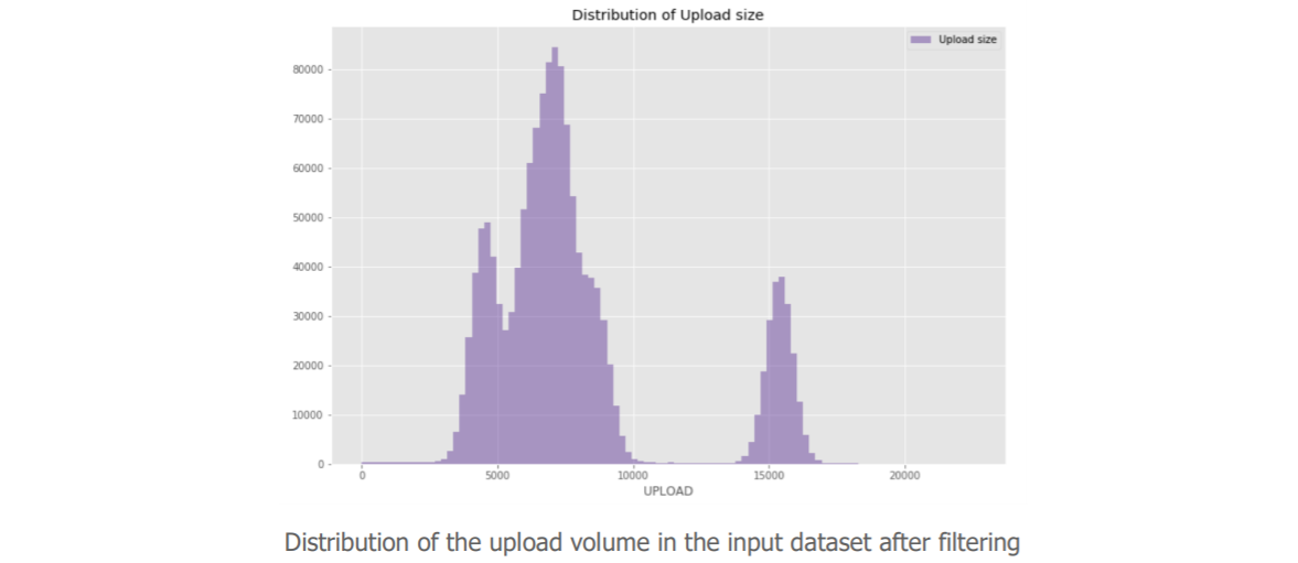
After several back and forth exchanges between data scientists challenging the data from a statistical point of view and cybersecurity teams responding with their professional eye, the data is simplified as much as possible. Data is then:
- Enriched by creating new variables that are denser in useful information. We introduced a relative upload volume to each site, measuring the difference between the upload volume of a request and its average value over the last 90 days. We could also add the connection time for example.
- Normalized by reducing the amplitude of each variable to decrease an over- or underweighting of certain variables.
- Digitized, as most algorithms can only interpret numerical variables.
We can now split our data set in two: one set that will be used to train our model, one set that will allow us to test its performance. Several separation methods exist, enabling us to keep certain characteristics of the data (e.g. seasonality), but the objective remains the same: to guarantee an evaluation measure as close as possible to the model’s real performances, by presenting the model with data that it did not have at its disposal during training.
Step 4: Choosing the learning method and training the model
Some algorithms are more efficient than others for a given problem, it is therefore necessary to make a reasoned choice.
There are two main categories of Machine Learning algorithms:
- Supervised, when we have labeled data as a reference to give as an example to our algorithm. These algorithms are for example used in cybersecurity by anti-spam solutions: they can learn via the users’ classification of emails as spam for example.
- Unsupervised, when we do not know precisely what we want to detect or when we lack examples to provide the algorithm with for its learning (i.e. we lack labeled data).
As explained above, the context of our use case points us more towards the second option. It is for the same reasons that we initially thought of Machine Learning. We then choose our unsupervised learning algorithm (Isolation Forest here, but we could have chosen another one) and train our model.
Step 5: Analyze results
We use our test data set to evaluate the effectiveness of our model in detecting exfiltration cases.
The designed model detects patterns in the data (queries), then compares the new data (queries) with these patterns and highlights those that deviate from what it considers to be the norm through its learning (anomaly score).
Here are our results:
« Ok, but how should I interpret all this ? »
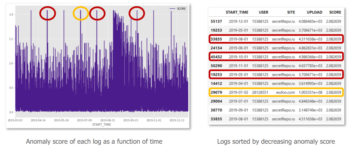
The graph on the left represents the anomaly scores associated with each query in the test set, sorted in chronological order. To the right are the logs with the highest anomaly scores.
After investigation with the cybersecurity business:
- The peak in yellow, corresponds to a much larger upload volume than others, from a user who extracts a large volume of data. This anomaly is legitimate. However, an alert based on a static volume per request rule would also have detected this suspicious communication.
- More interesting now, the peaks in red, correspond to requests for low volumes of regular uploads to unknown sites from the same user. These anomalies are harder to detect with conventional means, yet our algorithm has given them the same anomaly score as a large volume. They therefore become just as high a priority to qualify for our cybersecurity alert management teams.
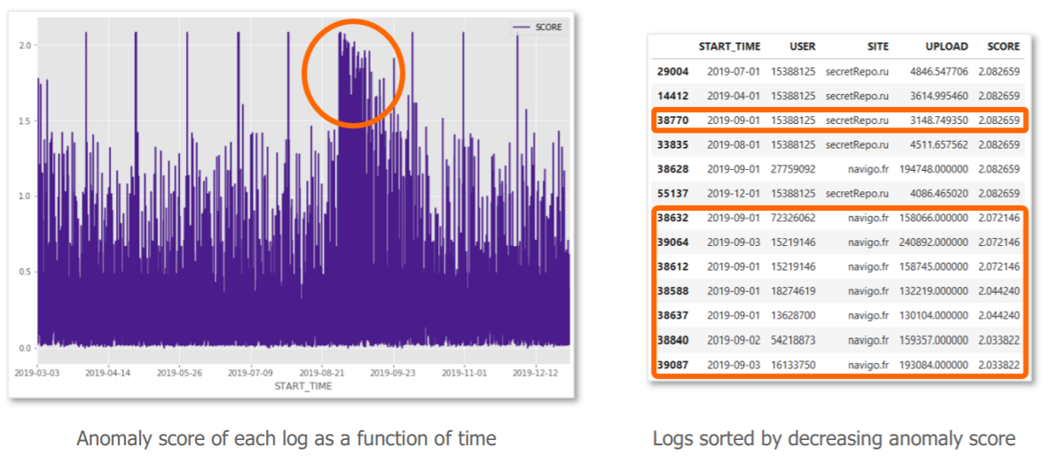
Now, let’s focus on the large package in the center of the graph (in orange). On the first day, we observe a large anomaly score, a sudden sending of data by many users to the city’s transit website. After investigation we realize that this is not a real security incident, but the annual sending of receipts for the continuation of transport subscriptions (we are at the beginning of September …). We then observe that the algorithm “understands” that these flows return to several users and progressively integrates them as a habit. The risk score therefore decreases day by day.
The model therefore detects what is out of the norm, regardless of the standard, and corrects itself with experience. This is where Machine Learning presents a real added value compared to traditional detection methods.
If the performance of the model on this first simplified use case attests to the potential value of the Learning Machine, it may be time to move on to step 6 – deployment to scale!
In a second article we will come back to these steps to highlight the success factors and pitfalls to be avoided when studying the possibilities of Machine Learning in cybersecurity.


